Why Isn’t 23andMe’s Disclaimer Good Enough?

23 and Me Spit Kit

[Image from 23andme.com]

The company 23andMe offers a different kind of ‘tech’ than I usually talk about on this blog, but it is meant to be a useful service for you (and for the company to collect information across many individuals).  Give them $100, and they will mail you a ‘spit kit’ with a tube that you literally spit in and send to it to them for analysis. They then use genotyping to determine whether you have certain variations in your DNA that are associated with your ancestry, disease, and other potentially genetically-derived traits.

I personally used their services about a year ago, mostly interested in ancestry.  Honestly, I wasn’t  too interested in their disease associations (though I believe this will become more and more useful as we sequence more individuals and develop better computational/statistical methods to analyze the data).  In the scientific community,  genetic associations with diseases are still, for good reason, met with skepticism (see, for example, this recent article).    This skepticism has worked its way up to politicians, resulting in various efforts to regulate laboratory developed tests.  I believe genetic testing and screening has a lot of potential and am excited that so many efforts exist to provide individuals with these kind of services, but as many scientists would probably agree, we are just beginning to understand how complex traits and diseases are associated with genetic variations across individuals.

23andMe recently received a letter from the FDA to “immediately discontinue marketing the PGS [Personal Genome Service] until such time as it receives FDA marketing authorization for the device”.

What surprised me when reading the letter was this statement:

Some of the uses for which PGS is intended are particularly concerning, such as assessments for BRCA-related genetic risk and drug responses (e.g., warfarin sensitivity, clopidogrel response, and 5-fluorouracil toxicity) because of the potential health consequences that could result from false positive or false negative assessments for high-risk indications such as these. For instance, if the BRCA-related risk assessment for breast or ovarian cancer reports a false positive, it could lead a patient to undergo prophylactic surgery, chemoprevention, intensive screening, or other morbidity-inducing actions, while a false negative could result in a failure to recognize an actual risk that may exist.

Perhaps because I have training in computational biology, I always assumed this information is meant to be more like a ‘hint’ or ‘suggestion’ that you might want to investigate a medical issue further with a physician who can conduct specialized follow-up tests and recommend further courses of action.  For instance, I have a minor version of Beta-thalassemia that apparently doesn’t require medication or affect my daily activities. 23andMe correctly identified that I have this trait.  This disorder can be discovered via blood testing by a physician, so if I didn’t already have these tests, my 23andMe report may have alerted me to investigate this further.   I think this is useful information.

My 23andMe page also displays this disclaimer:

The genotyping services of 23andMe are performed in LabCorp’s CLIA-certified laboratory. The tests have not been cleared or approved by the FDA but have been analytically validated according to CLIA standards. The information on this page is intended for research and educational purposes only, and is not for diagnostic use.

I do think that it could be made more prominent perhaps with a clause that states that some of these associations are in a stage of ‘early research’, but I am writing this post more to pose a general question to anyone that has some insight into the legal aspects of this recently newsworthy topic: why isn’t the disclaimer above (or a better one) good enough for the FDA?   Certainly, I understand that the general public doesn’t have the same knowledge I do about genetic tests, but given a disclaimer like this, why can’t 23andMe sell me their services and let me make follow-up decisions?

Some FDA links that are relevant:

Is clustering just an art?

Clustering data is the practice of grouping or partitioning a set of points based on how similar they are to one another.  One of the most basic forms of this would be by eye when looking at a plot of data.  For example, if we see two clumps on the x and y axes, then we say these data are grouped into two clusters.

plot(matrix(ncol=2,byrow=TRUE,jitter(c(rep(c(1,1),50),rep(c(2,2),50)))), xlim=c(.5,2.5), ylim=c(0.5,2.5),xlab=NA, ylab=NA)

plot(matrix(ncol=2,byrow=TRUE,jitter(c(rep(c(1,1),50),rep(c(2,2),50)))), xlim=c(.5,2.5), ylim=c(0.5,2.5),xlab=NA, ylab=NA)

Here, I artificially created two clusters in the R project tool grouped around (1,1), and (2,2).  The job of clustering tools is to figure out that these are indeed clusters.  This becomes harder when dealing with more than two dimensions, different types of data, and the question of what a cluster actually is.

Clustering tools are often used as a form of exploratory data analysis and fit within the class of unsupervised learning techniques. It’s not hard to see their practical relevance when they can help form groups from data elements having many different properties.

For some time now, I’ve heard the phrase “clustering is an art not a science.”  This becomes even more evident when faced with the frustrating quantity of clustering algorithms for specialized tasks and intimate interaction with the data to realize what’s actually happening.  Moreover, I can’t help sneaking suspicion on how certain techniques seem to overlap with one another. Now I’m not trying to knock specialized techniques.  In fact, quite the opposite.  For the thoughtful ones that seem to tackle a particular class of data, at least they do that and can be used.   That being said, without being able to formally lay out what’s actually happening, it’s hard to have a sound basis on which to compare methods.

What I’d like to (quickly) highlight in this post is a couple of interesting notions that tickle the possibility of a cleaner way to think about clustering. I’m not going to focus on the usual classifications of algorithmic approaches (e.g. hierarchical vs. partitioning).  While those distinctions are useful in choosing techniques and tools to cluster with, I think it might be valuable to look at the problem without concerning ourselves too much with traditional algorithms.

A data point can be quite flexible. It’ s just a tuple.  It can even be of mixed types (e.g. the first dimension can be some point in the real numbers, the second can be one of n nominal elements of a set, …).

All that matters is that we can define the distance between any two tuples. Even with mixed types, there are reasonable ways to approach this [1]. With this, we have a metric space.

We can stick this metric space in a Euclidean space. In the mid-80s, it was shown that any metric space with n elements (in our case tuples) can be embedded in a O(log n)-dimensional Euclidean space with some reasonable constraints on distortion [2]. Distortion is essentially the discrepancy between the true distances in the n element metric space and the distances in the Euclidean space. A decade later, randomized algorithms were developed to actually do this (e.g [3]).

The curse of dimensionality is a problem where the higher we go in dimension, the more likely it is for points to hover around the edges of some abstract hypersphere of our cluster.  This is because as the dimension increases, most of the volume of the hypersphere is contained in some small distance from the edge of the sphere.  Say our tuple was just a vector in the real number space, then it may be possible to reduce the dimensionality considerably and not bias our cluster shapes too much due to high dimension.

These facts (the first reference being quite practical and the last two more foundational) are quite relevant to clustering and I’d argue make the whole thing a little more of “a science” (eh hem, “a math”).

There are, I feel, two big issues I’ve ignored ’till yet, and these seem to really make up the “art” part.

1. We still have to take these points in some lower-dimensional Euclidean space and partition them into groups.  This requires some assumption of what a cluster actually is.  We can assume they’re spherical, but that’s likely not always the case.  What about different types of shapes?   While clustering shape sounds minor and in some cases may not be practically that relevant, to my knowledge, most ways of defining distances between clusters tend to restrict all the clusters to relatively homogeneous shapes.  This seems like a problem.  Maybe it can be dealt with mathematically in some way?

2. Let’s go back to the start where I talk about defining distances between points.  This can be a potentially arbitrary process depending on the methods by which the data was gotten in the first place.  But even aside from that, the structure one is clustering on may suggest a variety of alternate ways to define distance between two points.  For example, we can define the distance between two nodes on a graph in many ways (not just the shortest path).

While for the moment I’m certainly more at home as a “user/developer” of tools in this regard, here’s to theory.

——

[1] Kaufman L and Rousseeuw PJ.  Finding Groups in Data: An Introduction to Cluster Analysis. John Wiley & Sons (1990).
[2] Bourgain J. “On Lipschitz embedding of finite metric spaces in Hilbert space”. Israel Journal of Math 52, 46-52 (1985).
[3] Linial N, London E, and Rabinovich U. “The geometry of graphs and some of its algorithmic applications”. Combinatorica 15, 215-245 (1995).

Histograms and density estimation

It is a common practice in the statistical analysis of data to group the samples into bins or categories.  The goal is usually to extract some structure that is useful and often hidden from us when looking at direct plots of the sample set.

For instance, a time series plot of the change in stock price may appear erratic and contain no order, but observing the frequency of certain price-changes may help us realize that on average there is no change as well as give us an idea as to the practical bounds to how much the price will change.

The purpose of this note is to speak a little to the role of histograms in statistics and probability.   While a variety of complications arise when using them for the estimation of a probability density function, they serve as a very practical (and efficient) tool in exploratory data analysis and provide a grounding for other forms of density estimation.

Histogram Construction

  • For a given a sample, what bin does it belong to?
  • How many samples are in a given bin?
  • What is the numerical range or volume of a given bin?

From here forward, we consider data samples which can lie in some region of the real number line (e.g. integers, fractions, and roots of integers). We’ll represent a sample of numbers by the vector \mathbf{x}, say \mathbf{x}=(1.2, 3.002, 1, 1, 2).

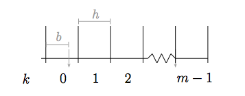
Basic histogramThe diagram outlines some relevant quantities of a histogram.  The minimum and maximum values of the sample (1 and 3.002 in the example above) help define the range that we will distribute our bins in.  We represent the bin width as h.  It is not required that a histogram have fixed-width bins, but this is one of the most commonly used and useful formulations.

The starting offset (0 \leq b < h) is also a useful quantity.  For instance, if the first bin starts at \min(\mathbf{x}) or b=0, any number falling in the range (\min(\mathbf{x}) \leq x < h) contributes to the quantity of elements in that bin.  For h=0.3, the range of the first bin in the example above is (1 \leq x < 1.3).  The two 1s and 1.2 will fall in the first bin.

Suppose we shift the bins a little to the left (i.e. b=0.1).  The range of the first bin is now (.9 \leq x < 1.2).  The two 1s fall in the first bin while 1.2 falls in the second.  So it is easy to see how both the bin width and offset affect our view of the histogram.

The total number of bins in a histogram can be represented as:

m=\left \lceil \frac{\max{(\mathbf{x})}-\min{(\mathbf{x}})}{h} \right \rceil + 1

where the \lceil x \rceil represents the next integer larger than x, and this follows analogously for \lfloor x \rfloor.  We add 1 to the traditional bin count to accommodate our offset b.

Integer bins in histogram

When constructing a histogram on a computer, we desire a function \text{bin}(x) that maps a sample to an appropriate bin index k=(0,1,\ldots,m-1).  Assuming that we begin the bins at 0, the bin index can be determined by dividing the sample from the bin width: \lfloor x/h \rfloor.  For h=0.3, it’s easy to see that numbers less than 0.3 will fall in bin 0, while a number twice as large will fall in the second bin, and so on.  Accounting for the offset, we have:

\text{bin}(x) = \left \lfloor \frac{x-\min{(\mathbf{x})}-b}{h} \right \rfloor

We also desire a function that will allow us to compute the start of the interval for a given bin index:

\text{interval}(k) = kh + \min{(\mathbf{x})}-b

The formulation above allows us to experiment with the two essential qualities of a histogram (bin width and offset) and it should be straightforward to see how this simple approach generalizes for multi-dimensional histograms of equal bin widths, except we then consider more generally the bin volume (e.g in the three-dimensional case the volume v=h^3).

In the terminology of computer science, these are constant time procedures.  If the bin widths are not fixed and arbitrarily set by the user then a more complicated method is required.  One can use a specialized function or binary search for finding the appropriate bin in this case [1].   Histograms can also accept a  variety of types (e.g. integers, single- or double-precision floating-point numbers) as inputs and if the compiler knows about this information ahead of time, it can optimize its code even further while providing a general interface of accumulators [2].

Histograms as density estimates

We now turn to a more mathematical perspective on histograms.  It is natural to treat a histogram as the estimation of a probability density function.  Once armed with the density function a variety of tools from probability and information theory are at our disposal, but we must take caution that the estimates of the density function hold true to the data sample and question whether we should be estimating the densities in the first place to solve the desired problem.

To get a taste for what this is like, we will derive the maximum likelihood estimator for a mathematical step function that represents the histogram.

Step function view of a histogram

Here, the function has m parameters: \mathbf{c}=(c_0,c_1,\ldots,c_{m-1}).  Provided our data sample and a given bin k, what is the optimal height, c_k^*, of the step function?

To find an estimate of the density function p_H(x; \mathbf{c}) we express the likelihood of our sample of data given the model parameters as:

\mathcal{L}(\mathbf{x}|\mathbf{c}) = \displaystyle \prod_{i=0}^{n-1}p_H(x_i; \mathbf{c}) = \displaystyle \prod_{k=0}^{m-1} c_k^{n_k}

Here, n_k represents the number of observed samples in bin k.  In other words, we’d like find c_k^* that maximizes the probability that we’ll find n_k items in bin k.  This optimization is subject to the density function constraint:

\displaystyle \sum_{k=0}^{m-1} c_k v_k = 1

where v_k is the volume of the given histogram region.

Constrained optimizations of this form can be solved using the method of Lagrange multipliers.  In this case, we have a multidimensional function:

f(\mathbf{c}) = \log \mathcal{L}(\mathbf{x}|\mathbf{c}) = \displaystyle \sum_{k=0}^{m-1} \log c_k^{n_k} = \displaystyle \sum_{k=0}^{m-1} n_k\log c_k

subject to the constraint that:

g(\mathbf{c})= 1- \displaystyle \sum_{k=0}^{m-1} c_k v_k = 0

Note that we took the log of the likelihood function so we can deal with sums rather than products.  This will come in handy when taking derivatives in a moment and is a common practice.

The gradient of a multidimensional function results in a vector field where each point–in our case represented by \mathbf{c}–has an associated vector of steepest ascent or descent on the multidimensional surface [3].  Our goal is to find where the steepest ascent of f(\mathbf{c}) is equal in magnitude and direction to that of g(\mathbf{c}).  This equality is represented as:

\nabla f(\mathbf{c}) = \lambda \nabla g(\mathbf{c})

And we can express this combined optimization with:

\nabla \Lambda(\mathbf{c}, \lambda) = \nabla f(\mathbf{c}) - \lambda \nabla g(\mathbf{c}) = 0

where \Lambda(\mathbf{c}, \lambda) is called the “Lagrangian”.  Computing the derivatives:

\frac{\partial \Lambda(\mathbf{c}, \lambda)}{\partial c_k} = \frac{n_k}{c_k} - \lambda v_k = 0

From this, we can see that

\frac{1}{\lambda}n_k = c_kv_k

Since \sum_{k=0}^{m-1} c_k v_k = 1 and \sum_{k=0}^{m-1} n_k = n, \lambda=n.  Thus our optimal height and estimate of the density is:

c_k^*= \hat{p}_H(x) = \frac{n_k}{nv_k}, \; \text{for all } x \text{ in bin } k

While this estimator is actually quite an intuitive result, it is important to observe that this only in the special case of step functions with varying volumes predefined.  What if, for example, we wanted to see what the best estimator is given a piecewise linear function or a spline between bins?  Or what if we want to find out what the bin volumes v_k should be as well?  This question motivates a general discussion on the estimation of the probability density function given the data sample \mathbf{x}, and these “data-driven” approaches are dubbed non-parametric [4].

Similar issues as those brought up in density estimation also arise in the estimation of mutual information [5].

—–

[1] Given a sample, start at the center-most bin.  If the sample is greater than that value, then start at the center most bin of the right half, otherwise do the same to the left.  Recurse this procedure until the desired bin is found.  The running time of this scales like \log_2(m).  The GNU scientific library provides utilities in this spirit

[2] See the C++ Boost Accumulator library for more information on this.

[3] For a more detailed tour of why this is as well as an intuitive contour plot geometrical interpretation of this, consult an introductory applied math text.  Setting f=c, we can study the function’s “surface contours”.  By definition, a vector \mathbf{x} along this contour does not change the value of f, therefore \nabla \cdot \mathbf{x} = 0.  Because of this, \nabla f must be normal to \mathbf{x}.

[4] Scott DW, Sain SR. “Multidimensional density estimation”. Handbook of Statistics: Data Mining and Computational Statistics 23. 297-306 (2004). Gentle JE. “Nonparametric estimation of probability density functions”. Elements of Computational Statistics. 205-231 (2002).

[5] Paninski L. “Estimation of entropy and mutual information”. Neural Computation 15. 1191-1253 (2003). Fraser AM, Swinney HL. “Independent coordinates for strange attractors from mutual information”. Physical Review A 33. 1334-1140 (1986).

R project map-reduce-filter tidbit

The R-project is a great tool set for statistical computing (this is its speciality) and even just to have around for quick calculations, plots [1], and data manipulations. The community is large and the source is open. It provides a nifty Unix-like environment to work in and is available on three major operating systems. </advertisement>

Because of the large community size and the highly-interpreted nature of the language, there is definitely an “impure” feeling about using it since some packages have procedures that will call their own C or Fortran code while others use the language directly. I personally like to see it as a good platform for exploratory data analysis/prototyping ideas, and like to leave the more heavy-lifting to something..different.

That said, since its internals are kind of Scheme-like, the expressiveness of the language for data manipulation in particular can be quite handy [2]. The introduction describes a function “tapply” which is useful for applying functions to groups of items with the same category. In that neighborhood there is also “lapply/sapply/mapply” [3] which are like the traditional “map” function. “subset” is very much like the traditional “filter” function.

Not-so-advertised are the “Map“, “Reduce“, and “Filter” functions (tricky-little capital letters). The differences between the traditional FP functions above and the two R analogs listed in the last paragraph are mostly conveniences for the way R treats its data.

If you use R or are interested in experimenting with it, keep these functions in mind because they can make just a few lines of code do some pretty awesome things.

——
[1] Gnuplot and matplotlib are also pretty good open source alternatives to plotting, and there are of course any non-open source options. In my opinion, experimentation with R is definitely worth the time if you’re playing with plots, and willing to side-step a bit from the Python bandwagon, since Python does have some well-developed statistical and scientific computing tools.

[2] See their “Manuals” section for some good introductory documentation and language definition. Many scripting languages these days support higher order functions.

[3] “mapply” is a neat sort-of multimodal map.

Monte carlo sampling the modularity space

Warning: I’m not really doing this entry justice, but it should be good-enough for logging purposes.

For the past few years, the complex networks community has spawned a thread in community detection: very roughly the problem of detecting subgraphs within a network that have a greater density of edges within-community than not.

Though greedy algorithms optimizing a very successful criteria called modularity (obviously there are many alternative methods to optimizing modularity overviewed in the literature) are good for very large networks, one side-issue is properly analyzing the variety of partitions that could be generated that have similar modularities. This has been explored a bit (too many links for the spirit of this post).

One way to tackle this issue is to use a technique called Markov Chain Monte Carlo (MCMC), in which the transition probabilities in your Markov chain are from one possible partitioning of the network to another. Since the number of possible partitions of n nodes in the network is equivalent to the number of possible set partitions with n members, we can’t possibly exhaustively explore the entire space for even moderately sized networks. But we can, if careful, sample from this space with proportional to a bias of our choice because it can be shown that the Markov chain will eventually reach a state of equilibrium.

This technique, among other things, helps us learn more about the properties of the space of partitions as well as analyze whether the partitioning buys us much (i.e. if the nodes really stay in one partition a lot or not for the ensemble of partitions generated at equilibrium). I’ve come across and have been pointed to literature where it’s in statistics, quantum chemistry, and statistical physics, and am most certain it’s used in many more fields of study. Part of the appeal in using the technique is that it allows for a surprising amount of flexibility in choosing the transition probabilities and is conceptually easy to grasp (I wonder how badly it’s abused).

I can now link you to some code I wrote.

It uses the same transition scheme described in Massen-Doye ’06, but samples directly proportional to the modularity rather than via parallel tempering on the Boltzmann distribution (an exploratory suggestion from Aaron Clauset). The results show that this works quite well itself, and the modularity of the partitions at equilibrium usually hover below the maximum determined modularity, as expected.

With this “starting point” (the cleaned up code) I have tried a variety of other transition schemes as well as done some thinking on what would be valuable in terms of the target distribution. This exploration serves as a good basis for continuing to play with modularity, its connection to hierarchical structure, and even dynamical systems.

On a less technical level, I have been slowly gathering notes on what’s actually happening (a.k.a WAH?) in the field of statistical analysis of complex networks (both static and dynamic) as a whole and what certain analysis techniques buy us for particular networks. Right now I’m still engrossed in seminal work, but as they become more refined I’ll post a link to them so that I can perhaps get more feedback on my “worldview” of the area.

And even more tangentially related, those of you who may reproducing research, there is a slight error in the reporting of the modularity of the karate club network for the fast algorithm (the author has been aware of this) and that the second pass of the CNM algorithm should be run at step MAXQ-1 to get the partition with optimal modularity.